

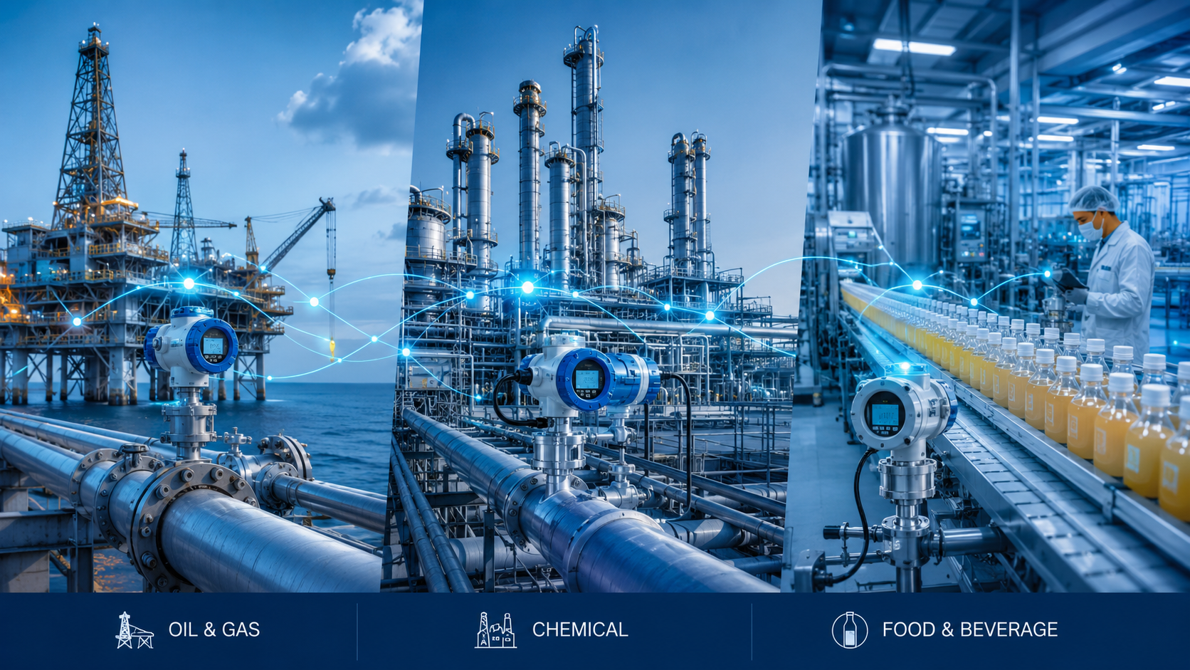
If you have ever dealt with process density measurement, you have probably come across tuning fork density meters at some point. They show up in refinery pipelines, chemical reactors, food production lines, pharmaceutical mixing tanks and a dozen other places where knowing exactly what is inside a pipeline matters.
The concept sounds simple enough on the surface. But once you dig into how the technology actually works, it is surprisingly elegant and worth understanding properly before you commit to a specific model or brand.
So let us walk through the complete working principle, step by step.
What Exactly Is a Tuning Fork Density Meter?
Before getting into the mechanics, it helps to be clear about the terminology. The name comes from the physical shape of the sensing element: two parallel prongs that look exactly like a musical tuning fork.
These prongs are not decorative. They are the actual measurement mechanism. When immersed in a liquid, their vibration frequency changes in a predictable, measurable way that correlates directly to the density of that liquid.
The instrument sends an electrical signal to a piezoelectric ceramic driver on one prong, which makes it vibrate. The other prong acts as a listener, picking up the vibration and feeding it back in a self-sustaining loop. That is the core of the entire system.
The 5-Step Working Principle
Here is where it gets more specific. The complete measurement cycle can be broken down into five distinct steps.
Step 1 — The Fork Gets Driven
A piezoelectric ceramic element sits attached to the tuning fork prongs. When electrical current is applied, the ceramic changes shape slightly, pushing one prong back and forth.
Think of it like pushing a child on a swing. You do not need to push constantly. You push at just the right moment in each cycle to keep the motion going. The electronics do exactly that, applying force at the natural resonant frequency of the fork.
This self-excited oscillation is what makes the system stable and responsive at the same time.
Step 2 — The Fork Vibrates in the Liquid
The prongs are inserted into the process liquid through a process connection, typically a threaded or flanged port on a pipeline or tank. They vibrate at their natural frequency while submerged.
This is the critical interaction point. The frequency at this stage is not fixed. It changes based on two things at the same time: the density of the liquid and the viscosity of the liquid.
Most modern instruments have algorithms that compensate for viscosity effects, isolating the density signal from the frequency output. Older or simpler models sometimes require manual viscosity correction, which adds complexity.
Step 3 — Frequency Gets Measured
The receiving prong picks up the vibration and converts it back into an electrical signal. The instrument measures the oscillation frequency with high precision, typically down to a fraction of a Hertz.
The relationship between frequency and density is inverse: a higher frequency means a lower density, and a lower frequency means a higher density. This is because denser liquids dampen the vibration more effectively, slowing the fork down.
The actual frequency range varies by design. A typical fork in water-based liquids might vibrate somewhere around 110 to 130 Hz. Move it into a denser liquid like heavy fuel oil, and the frequency drops noticeably.
Step 4 — Calibration Curve Converts Frequency to Density
The raw frequency number alone is not useful until it is converted into a density reading. That conversion relies on a calibration curve established during factory testing.
At the factory, the instrument is immersed in a series of reference liquids with known densities, usually at a standard temperature. The frequency output at each reference point is recorded and a curve is fitted from these data pairs.
In most modern instruments, this curve is stored digitally in the transmitter electronics. The instrument applies it in real time, outputting a direct density reading rather than a raw frequency.
Temperature matters a lot at this stage. Density is strongly temperature-dependent. A liquid that reads 1.000 g/cm³ at 20°C might read 0.995 at 25°C even if nothing else changed. Good instruments handle this with built-in temperature compensation.
Step 5 — Signal Gets Sent to the Control System
The final density reading is output in a standard industrial format. The most common is a 4-20mA current loop, which is familiar to virtually any distributed control system or PLC.
Some instruments also offer RS485 digital communication using the Modbus protocol. This allows multiple instruments to be networked together on the same bus, with richer data available including diagnostics and configuration information.
The choice between 4-20mA and Modbus comes down to your existing infrastructure and how much data you need in real time.
Frequency, Density and Temperature: The Three Variables
Understanding the relationship between these three is what separates someone who just reads a display from someone who can actually interpret the data correctly.
The resonant frequency of the fork is a function of the liquid is density and the fork is physical properties. Denser liquids cause the fork to vibrate more slowly. Higher temperatures change both the liquid density and the fork is material properties, so temperature compensation is not optional in most applications.
This is also why the viscosity limit exists. Very viscous liquids, above roughly 2000 centipoise for most instruments, start to interfere with the fork is ability to vibrate freely. For high-viscosity applications, a rotational viscometer or a different technology is usually more appropriate.
Common Installation Mistakes That Can Wreck the Signal
Understanding how the instrument works is only part of the story. If the fork is not properly immersed, if there are air bubbles trapped on the prongs, or if it is installed directly downstream of a pump or a sharp elbow, the frequency signal will be noisy or just wrong.
A few practical rules to keep in mind:
Always keep the fork fully submerged. Running the instrument with the prongs out of the liquid, even briefly, can damage the piezoelectric element.
Avoid placing the instrument immediately after a pump or a pipe elbow. The turbulence will introduce noise into the frequency signal.
Make sure the process connection is oriented correctly. Some forks are designed for vertical insertion only.
Check for buildup or scaling on the prongs if the liquid is prone to deposits. Anything stuck to the fork changes its effective mass and therefore its frequency response.
What Makes a Good Tuning Fork Density Meter
Not all instruments are created equal, even if they all follow the same fundamental principle. The differences that matter most in the field come down to a few practical details.
| Specification | What to Look For |
| Temperature compensation | ±0.1°C accuracy or better for precise density correction across process temperature ranges |
| Wetted materials | 316L stainless steel as standard; Hastelloy or Tantalum for aggressive chemicals |
| Output options | 4-20mA as baseline; RS485/Modbus RTU for diagnostics and multi-device networking |
| IP rating and protection | IP67 minimum for outdoor or washdown environments; ATEX/IECEx for hazardous areas |
| Maintenance design | Remote transmitter separates electronics from process wetted parts for field replacement without breaking the pipe |
| Viscosity limit | Check maximum operating viscosity; typically 2000 cP for standard tuning fork designs |
Why Engineers Still Choose This Technology
Despite the availability of Coriolis meters, nuclear gauges and ultrasonic density measurement options, tuning fork density meters remain one of the most widely used technologies in inline process density measurement.
The reasons are mostly practical:
The sensing element is physically small and simple. There are no moving parts in the traditional sense, no radiation sources, and no optical windows that can get dirty or scratched.
Response time is fast, typically settling to within specification in a few seconds.
Installation is straightforward using standard pipe fittings.
Cost of ownership over time tends to be lower than Coriolis meters for many applications, particularly when liquid viscosity falls within the instrument is range.
Maintenance is relatively simple compared to other technologies.
The LONNMETER LONN700 Series in Practice
For engineers evaluating options, the LONNMETER LONN700 inline tuning fork density meter represents one of the more complete implementations of this technology. It covers the measurement range most commonly needed in industrial applications, with factory calibration against traceable reference standards.
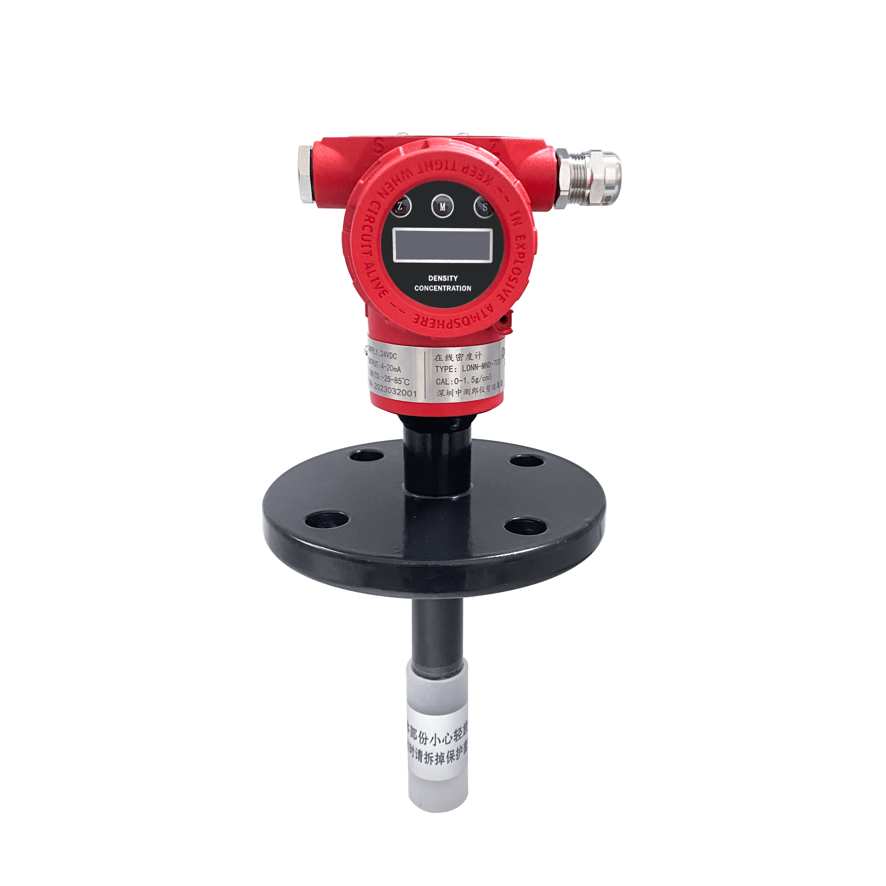
The instrument uses a remote transmitter design, meaning the electronics are housed in a separate enclosure from the process wetted parts. This makes field replacement straightforward without breaking the process connection.
Available output options include 4-20mA and RS485 with Modbus RTU protocol, covering most DCS and PLC integration requirements. The standard temperature compensation range handles most common process conditions without additional configuration.
Accuracy specification is ±0.002 g/cm³, well within the tolerance required for most refining, chemical and food processing applications. The remote transmitter design also reduces heat transfer from the process to the electronics, which contributes to long-term stability over years of continuous operation.
If you want to see the full specifications or discuss a specific application, the LONNMETER technical team can work through the details based on your process parameters.
Post time: May-25-2026


